Probability & Statistics

Probability

Bayes' Theorem
Two events A and B are mutually exclusive if $P(A\cup B)=0$. Two events A and B are independent if $P(A\cup B)=P(A)P(B)$. Therefore, two mutually exclusive events A and B are independent if and only if $P(A)=0$ or $P(B)=0$.

Expected value of random variable $$ \mathbb{E}[X]=\sum X_i \cdot p(X_i) $$
Probability distributions
- Discrete
  - Bernoulli => binomial, geometric
    - Bernoulli: e.g. flip a coin
    - Binomial: the probability that there are $k$ successes out of $n$ trials in a series of repeated Bernoulli trials meeting three criteria $$ p_X (k)= {n \choose k}p^k (1-p)^{n-k} $$
      - Fixed number of trials $n$
      - Indepedent trials
      - Constant probability of success
    - Geometric: the probability that the first $k-1$ trials are failures im repeated Bernoulli trials $$ p_X (k)=(1-p)^{k-1}p $$
      - Expected value of a geometric distribution: $$ \mathbb{E}(X)=\frac{1}{p} $$
  - Poisson => exponential (continuous)
    - Poisson: the probability of observing $k$ events in a time period given the length of the period and the average events per time
- Continuous

Permutations & Combinations

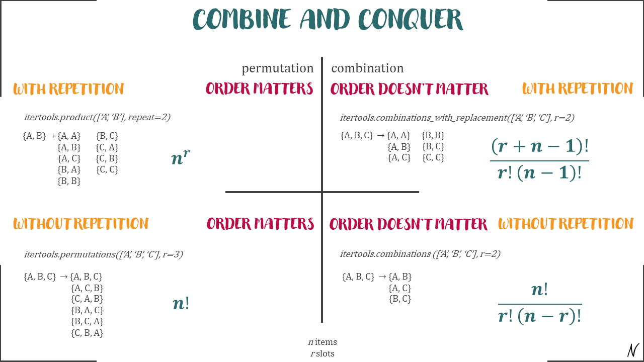
Without Replacement

Product rule: if an experiment has $N_1$ outcomes for the first stage, $N_2$ outcomes for the second stage, ..., and $N_M$ outcomes for the $M$th stage, then the total number of outcomes of the experiment is $$ N_1 \times N_2 \times \cdots N_M $$
Permutations: the number of orderings of $N$ distinct objects is $$ N! $$
- A permutation is an act of arranging the objects or numbers in order
Combinations are the way of selecting the objects or numbers from a group of objects or collection, in such a way that the order of the objects does not matter
Permutations of $n$ distinct objects: $$ P(n)=n! $$
$k$-permutations: permutations of $k$ items taken from $n$ distinct objects (order matters): $$ P(n,k)=\frac{n!}{(n-k)!} $$
Combinations of $k$ items taken from $n$ distinct objects ($n$ choose $k$) (order doesn't matter): $$ C(n,k)=\frac{n!}{k!(n-k)!} $$

$$ C(n,k) = C(n,n-k) $$

Multinomial coeffficients: if we have $k$ types of objects ($N$ total), with $N_1$ of the first type, $N_2$ of the second, ..., and $N_k$ of the $k$th, then the number of arrangements possible is $$ C(N,N_1)C(N-N_1,N_2)\cdots C(N_k,N_k)=\frac{N!}{N_1!N_2!\cdots N_k!} $$
- E.g. anagrams (how many ways can you arrange the letters in a word like "mississippi"?) $$ \frac{11!}{4!4!2!} $$

With Replacement

$k$-combinations with repetition
- Divider problem
The number of ways to distribute $n$ indistinguishable balls into $k$ distinguishable bins is $$ {n+(k-1) \choose k-1} = {n+(k-1) \choose n} $$
- This is the same as having $k$ types of objects, i.e. $n$-combinations with repetition

Distiguishable vs Indistinguishable

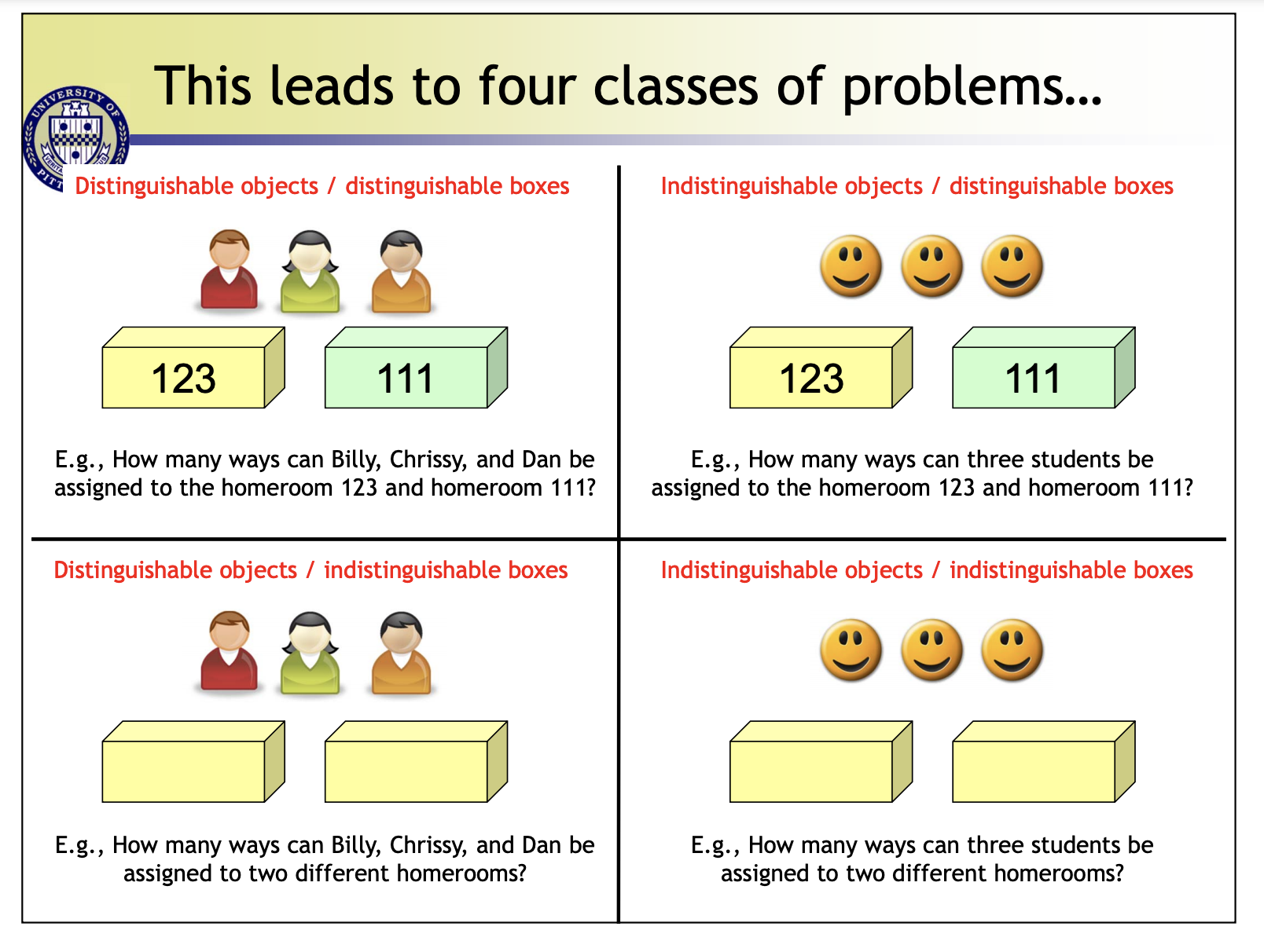
The number of ways that $n$ distinguishable items can be placed into $k$ distinguishable boxes so that $n_i$ objects are placed into box $i$ ($1\leq i\leq k$) is $$ C(n,n_1)C(n-n_1,n_2)\cdots C(n-n_1-\cdots -n_{k-1},n_k)=\frac{n!}{n_1!n_2!\cdots n_k!\cdot (n-n_1-n_2-\cdots -n_k)!} $$

The number of ways that $n$ indistinguishable items can be placed into $k$ distinguishable boxes is the same as counting the $n$-combinations for a set with $k$ elements when repetition is allowed
1. Treat our indistinguishable items as *s
2. Use | to divide our distinguishable bins
3. Count the ways to arrange $n$ placeholders and $k-1$ dividers
- There are $C(n + k – 1, n)$ ways to place $n$ indistinguishable objects into $k$ distinguishable boxes

The number of ways that $n$ distinguishable items can be placed into $k$ indistinguishable boxes can be described as Sterling number of the second kind

The number of ways that $n$ indistinguishable items can be placed into $k$ indistinguishable boxes has no closed formula

Statistics

Central Limit Theorem: the sampling distribution of the sample means approaches a normal distribution as the sample size gets larger (>30)
Power
Type I error vs Type II error:
p value
Confidence interval

Machine Learning Fundamentals

Dimensionality Reduction

Curse of dimensionality: high dimensional data leads to problems such as data sparsity and distance concentration
- Data sparsity: the training samples available for building the model may not capture all possible combinations of the attributes; in real-time when less frequently occurring combinations are fed to the model, it may not predict the outcome accurately
- Distance concentration: all the pairwise distances between different samples/points in the space converging to the same value as the dimensionality of the data increases
Drawbacks of dimensionality reduction:
- Can be computationally intensive
- It can be hard to interpret the transformed independent variables
- As we reduce the number of features, some information is lost, due to which the performance of the algorithms degrades

Feature Elimination

Feature Extraction

PCA

What is PCA?
- It is a dimensionality reduction technique which summarizes a large set of correlated variables (basically a high dimensional data) into a smaller number of representative variables, called the principal components, that explains most of the variability in the original set.
- Preserves as much information as possible
When to use PCA?
- Do you want to reduce the number of variables, but aren’t able to identify variables to completely remove from consideration?
- Do you want to ensure your variables are independent of one another?
- Are you comfortable making your independent variables less interpretable?
Standardizing (mean 0 and variance 1) is important for PCA because it is looking for a new orthogonal basis where the origin stays the same, so having your data centered around the origin is good. The first principal component is the direction with the most variance, by scaling a certain feature with a weight of more than 1 will increase the variance on this axis and thus give more weight to this axis (reference)

ML Methods

Stanford CS229 Cheat Sheet

Discriminative vs generative models
- Discriminative models: to obtain prediction for a data point, the model computes the probability of the data point belonging to each class; the class with the highest probability wins
Linear vs non-linear models
Closed-form solution vs iterative methods (e.g. gradient descent, Newton's Method, etc)
- Cross Validated: Solving for regression parameters in closed-form vs gradient descent
- Closed-form solution is expensive when the data size is large, etc

Supervised Learning

Linear Regression

Linear model
Has closed-form solution

Logistic Regression

Linear model
Has closed-form solution

Support Vector Machines (SVMs)

Definitions and Key Distinctions

Support Vector Machines (SVMs) is a supervised machine learning for classification tasks where the model learns an optimal hyperplane (i.e. a decision boundary) that maximizes margins
Support vectors: data points that lie closest to the decision surface or hyperplane
Only a subset of points (i.e. support vectors) influence the choice of hyperplane, rather than all data points (in the case of logistic regression, neural nets, etc)
The use of kernels
**"Kernel trick"**: we can avoid expensive operations in high dimensions by finding an appropriate kernel function $K(x, z)$ that is equivalent to the inner product of the feature map ($\phi$, which maps attributes $x$ ($x\in \mathbb{R}^d$) to $\phi(x)$ ($\phi(x) \in \mathbb{R}^p$) in higher dimensional space)

Additional Info

SVMs can be reframed as an optimization problem aiming to minimize $\frac{1}{2} \vert\vert w\vert\vert$
Can be linear or non-linear (depending on the kernel function)
- Linear SVM: data points can be easily separated with a linear line
- Non-linear SVM: data points cannot be easily separated with a linear line
Can be used for both classification and regression (as well as outliers detection) (reference)
- Support Vector Regression: SVR finds a line (i.e. a hyperplane) to fit the dataset (rather than to separate the data points) and fit the errors within a certain threshold (i.e. $\epsilon$)
The intuition behind maximizing the margin is that this will give us a unique solution to the problem of finding $f(x)$ and also that this solution is the most general under these conditions, i.e. it acts as a regularization. (reference)
In a feature space of dimension $N$, if $N>n$ then there will always be a separating hyperplane. However this hyperplane may not give rise to good generalization performance, especially if some of the labels are incorrect. (reference: Gaussian Processes for Machine Learning)

Pros & Cons

Pros:
- Effective in high dimensional spaces (& when the number of features is greater than the number of examples)
  - Why is this true?
  - Stackoverflow: How to approach machine learning problems with high dimensional input space?
- Works well in smaller, cleaner datasets
- Can be used to model non-linear relationships via the use of kernels
Cons:
- Isn’t suited for larger datasets as the training time with SVMs can be high

$k$-Nearest Neighbors

A non-parametric approach where the response of a data point is determined by the nature of its $k$ neighbors from the training set
Can be used in both classification and regression
The higher the parameter $k$, the higher the bias; the lower the parameter $k$, the higher the variance

Gaussian Discriminant Analysis

Generative model
Assumptions:
- $y \sim \text{Bernoulli} (\phi)$
- $x\vert y=0\sim \mathcal{N}(\mu_0, \Sigma)$
- $x\vert y=1\sim \mathcal{N}(\mu_1, \Sigma)$

Naive Bayes

Generative model
Assumptions:
- Independent predictors, i.e. $$ P(x\vert y)=P(x_1, x_2, ... \vert y)=P(x_1\vert y)P(x_2\vert y)...=\prod_{i=1}^n P(x_i\vert y) $$
Widely used for text classification and spam detection

Decision Trees

Non-linear model
Decisions trees are very sensitive to the data they are trained on; small changes to the training set can result in significantly different tree structures $\to$ bagging
Random forest: a tree-based ensemble technique that uses a high number of decision trees built out of randomly selected sets of features; contrary to the simple decision tree, it is highly uninterpretable
Boosting:
- Adaptive boosting: e.g. Adaboost
- Gradient boosting: e.g. XGBoost

Unsupervised Learning

$k$-Means

Pros:
- Easy to implement
- With a large number of variables, may be computationally faster than hierarchical clustering (linear time complexity, i.e. $O(n)$)
Cons:
- Difficult to predict the number of clusters
- Initial seeds may have strong impact on final results
- The order of data has an impact on results
- Sensitive to scale (normalizing / standardizing data may lead to different results)
- Works well when the shape of clusters are hyper-spherical (or circular in 2 dimensions). If the natural clusters occurring in the dataset are non-spherical then $k$-means is probably not a good choice

Hierarchical Clustering

Pros:
- Hierarchical structure is more informative & makes it easier to decide on the number of clusters by looking at the dendrogram
- Easy to implement
Cons:
- Not suitable for large datasets (quadratic time complexity, i.e. $O(n^2)$
- Initial seeds may have strong impact on final results
- The order of data has an impact on results
- Sensitive to outliers

Gaussian Mixture

Advanced ML Methods

Ensemble

The low correlation between models is the key (protect each other from individual errors)

Bagging

Given a dataset, instead of training one classifier on the entire dataset, you sample with replacement to create different datasets, call bootstraps, and train a classification or regression model on each of these bootstraps
A random forest is an example of bagging (random forest = bagging + feature randomness)

Boosting

Each learner in the ensemble is trained on the same set of samples but the samples are weighted differently among iterations. Thus, future weak learners focus more on the examples that previous weak learners misclassified
The final classifier is a weighted combination of the existing classifiers - classifiers with smaller training errors have higher weights
An example of a boosting algorithm is Gradient Boosting Machine (XGBoost, LightGBM)
Gradient boosting vs adaptive boosting
- In Gradient Boosting, "shortcomings" (of existing weak learners) are identified by gradients
- In Adaboost, "shortcomings" are identified by high-weight data points
  - Disadvantages
    - Adaboost cannot be parallelized since each predictor can only be trained after the previous one has been trained and evaluated

High Dimensional Data

Which Models Require Normalization / Standardization of Data?

Deep Learning

An overview of gradient descent optimization algorithms KDnuggets: Deep Learning's Most Important Ideas

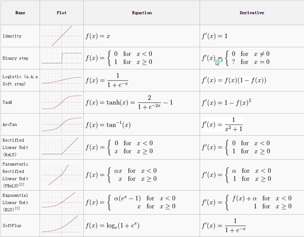
Activation Functions

The purpose of the activation function is to introduce non-linearity into the output of a neuron
Binary step function
- Only suitable for binary classes
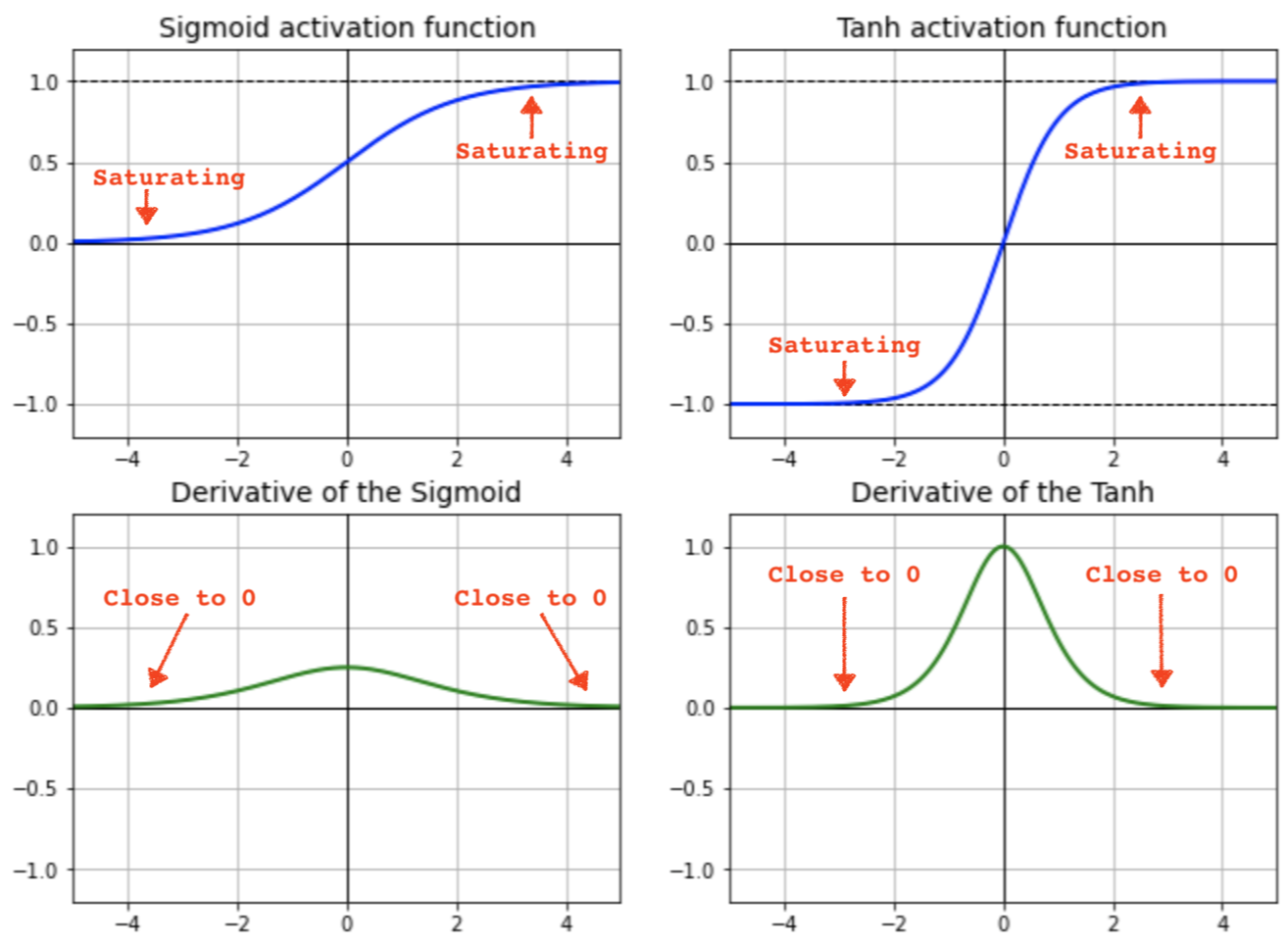
Sigmoid
- Prone to vanishing gradient
Tanh
- Prone to vanishing gradient
ReLU (reference)
- Pros:
  - ReLU takes less time to learn and is computationally less expensive than other common activation functions
  - Because it outputs 0 whenever its input is negative, fewer neurons will be activated, leading to network sparsity and thus higher computational efficiency
  - Tanh and sigmoid functions are prone to the vanishing gradient problem, where gradients shrink drastically in backpropagation such that the network is no longer able to learn. ReLU avoids this by preserving the gradient since:
    (i) its linear portion (in positive input range) allows gradients to flow well on active paths of neurons and remain proportional to node activations
    (ii) it is an unbounded function (i.e., no max value)
- Dying ReLU: when many ReLU neurons only output values of 0 because the inputs are in the negative range; when most of these neurons return output zero, the gradients fail to flow during backpropagation, and the weights are not updated
- How to solve the dying ReLU problem?
- The dying ReLU is a kind of vanishing gradient (reference)
  - Lower learning rate
  - Leaky ReLU
  - Randomized asymmetric initialization instead of symmetric probability distributions (i.e. He initialization)
Leaky ReLU
Softmax

Gradient Descent

Gradient ascent vs gradient descent
Gradient descent: based on a convex function and tweaks its parameters iteratively to minimize a given function to its local minimum
Why do we update parameters in the direction opposite of the gradient?
- Gradient is the direction of the greatest change of a scalar function
- Think about $y=x^2$, with gradient $y'=2x$, but we need to find the local minima; similarly for $y=-x^2$, with gradient $y'=-2x$, we need to find local maxima
Variants of gradient descent:
- Batch gradient descent (vanilla gradient descent) (reference):
  - Computes the gradient of the loss function for the entire training dataset
    - No need to shuffle the training data because we're using the entire training dataset to make a single update
  - Pros:
    - Can benefit from vectorization
    - Produces a more stable gradient descent convergence than SGD
  - Cons:
    - Sometimes a stable error gradient can lead to local minima and unlike stochastic gradient descent, no noisy steps are there to help to get out of the local minima
    - The entire training set can be too large to process in the memory
    - Doesn't allow for updating the model online (i.e. with new examples on the fly)
- SGD (reference)
  - Performs a parameter update for each training example
  - Pros:
    - Easier to fit in the memory due to a single training example being processed by the network
    - Computationally fast as only one sample is processed at a time
    - For larger datasets, it can converge faster as it causes updates to the parameters more frequently
    - Due to frequent updates, the steps taken towards the minima of the loss function have oscillations that can help to get out of the local minimums of the loss function
    - Can be used to learn online
  - Cons:
    - Due to frequent updates, the steps taken towards the minima are very noisy and it may take longer to converge
    - Frequent updates are computationally expensive because of using all resources for processing one training sample at a time
    - It loses the advantage of vectorized operations as it deals with only a single example at a time
    - Performs redundant computations for large datasets, as it recomputes gradients for similar examples
    - complicates convergence to the exact minimum, as SGD will keep overshooting
- Mini-batch gradient descent:
  - Mini-batch gradient descent takes the best of both worlds

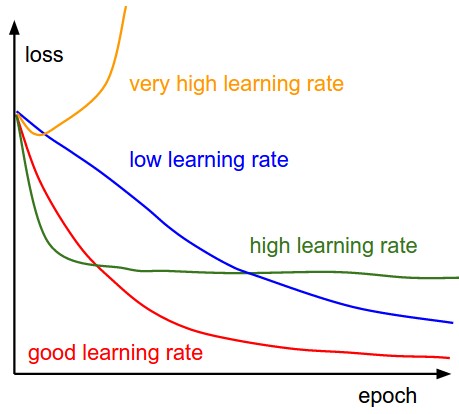
Learning Rates

First step to combatting non-convergence: learning rate schedules
Challenges with vanilla gradient descent (reference)
- A learning rate that is too small leads to painfully slow convergence, while a learning rate that is too large can hinder convergence and cause the loss function to fluctuate around the minimum or even to diverge
- Learning rate schedules try to adjust the learning rate during training by e.g. annealing, i.e. reducing the learning rate according to a pre-defined schedule or when the change in objective between epochs falls below a threshold. These schedules and thresholds, however, have to be defined in advance and are thus unable to adapt to a dataset's characteristics
- Additionally, the same learning rate applies to all parameter updates. If our data is sparse and our features have very different frequencies, we might not want to update all of them to the same extent, but perform a larger update for rarely occurring features
- The presence of saddle points (points where one dimension slopes up and another slopes down), which makes it notoriously hard for SGD to escape, as the gradient is close to zero in all dimensions

Optimizers

Responsible for figuring out how to adjust the parameters of the network to make it learn the objective
SGD
Momentum
- SGD has trouble navigating ravines, i.e. areas where the surface curves much more steeply in one dimension than in another
- Momentum is a method that helps accelerate SGD in the relevant direction and dampens oscillations. It does this by adding a fraction $\gamma$ of the update vector of the past time step to the current update vector
- Think of momentum as pushing a ball down a hill. The ball accumulates momentum as it rolls downhill, becoming faster and faster on the way
Adagrad
- It adapts the learning rate to the parameters, performing smaller updates (i.e. low learning rates) for parameters associated with frequently occurring features, and larger updates (i.e. high learning rates) for parameters associated with infrequent features
- Strengths:
  - Well-suited for sparse data
  - Eliminates the need to manually tune the learning rate
- Weaknesses:
  - Accumulation of the squared gradients in the denominator: since every added term is positive, the accumulated sum keeps growing during training. This in turn causes the learning rate to shrink and eventually become infinitesimally small, at which point the algorithm is no longer able to acquire additional knowledge
Adadelta
- An extension of Adagrad that seeks to reduce its aggressive, monotonically decreasing learning rate
- Instead of accumulating all past squared gradients, Adadelta restricts the window of accumulated past gradients to some fixed size $w$
- No need to set a default learning rate as it has been eliminated from the update rule
RMSprop
- Similar to Adadelta
Adam (Adaptive Momentum Estimation)
- In addition to storing an exponentially decaying average of past squared gradients $v_t$ like Adadelta and RMSprop, Adam also keeps an exponentially decaying average of past gradients $m_t$, similar to momentum
- Adam, or adaptive momentum, combines two ideas to improve convergence: per-parameter updates which give faster convergence, and momentum which helps to avoid getting stuck in saddle point.

Data

Shuffling

We want to avoid providing the training examples in a meaningful order to our model as this may bias the optimization algorithm. Consequently, it is often a good idea to shuffle the training data after every epoch
On the other hand, for some cases where we aim to solve progressively harder problems, supplying the training examples in a meaningful order may actually lead to improved performance and better convergence
Not needed for batch gradient descent

Data Augmentation

Reduces the chances of overfitting
While data augmentation does have an explicit regularization effect, exploiting it can actually lead to the model not learning enough resulting in poor prediction results (reference) #### Data Leakage

Model Components

Batch Normalization

Batch normalization is designed to combat "internal covariate shift" (change in the distribution of inputs during training)
Standardizes layer outputs so that assumptions the subsequent layer makes about the spread and distribution of inputs during the weight update will not change
Reduces training time

Dropout

During training, individual nodes are ignored with probability $1-p$ or kept with probability $p$
Dropout helps prevent overfitting due to a layer's "over-reliance" on a few of its inputs. Because these inputs aren't always present during training (i.e. they are dropped at random), the layer learns to use all of its inputs, improving generalization (reference) (a layer's "over-reliance" on a few of its inputs has the effect of co-dependency among neurons, i.e. neurons developing redundant representations of data for prediction)
A single model can be used to simulate having a large number of different network architectures by randomly dropping out nodes during training
There are several (related) explanations to why dropout works. It can be seen as a form of model averaging — at each step we “turn off” a part of the model and average the models we get. It also adds noise, which naturally has a regularizing effect. It also leads to more sparsity of the weights and essentially prevents co-adaptation of neurons in the network. (reference)
Increases trianing time

Vanishing Gradients

Vanishing gradient problem arises in cases where the gradient of the activation function is very small. During back propagation when the weights are multiplied with these low gradients, they tend to become very small and “vanish” as they go further deep in the network. This makes the neural network to forget the long range dependency
Generally a problem in cases of recurrent neural networks where long term dependencies are important (reference)
Sigmoid and tanh are prone to vanishing gradients; ReLU partially solves the problem (unbounded on the positive side, dying ReLU on the negative side; use leaky ReLU or different initialization method or batch normalization

Exploding Gradients

Results inn an overflow value (or NaN) in the weights
Can be solved by gradient clipping

Weight Initialization

If all the neurons have the same value of weights, each hidden unit will get exactly the same signal. While this might work during forward propagation, the derivative of the cost function during backward propagation would be the same every time.
In the 1-layer scenario, however, the cost function is convex (linear/sigmoid) and thus the weights will always converge to the optimal point, regardless of the initial value (convergence may be slower)

Model Architectures

CNNs

Unlike a regular Neural Network, the layers of a ConvNet have neurons arranged in 3 dimensions
Why are CNNs primarily used for computer vision tasks?
- The key lies in the convolution operation
- The primary purpose of Convolution in case of a CNNs is to extract features from the input image. Convolution preserves the spatial relationship between pixels by learning image features using small squares of input data.
- Less likely to overfit because CNNs typically have a lot more parameters
Filters
Pooling
- The result of using a pooling layer and creating down sampled or pooled feature maps is a summarized version of the features detected in the input. They are useful as small changes in the location of the feature in the input detected by the convolutional layer will result in a pooled feature map with the feature in the same location. This capability added by pooling is called the model’s invariance to local translation. (reference)
Padding
Convolutional layers are locally connected layers with shared weights
- Parameter sharing
- Local connectivity
  - Each neural is connected only to a subset of the input image (unlike a neural network where all the neurons are fully connected)
- This helps to reduce the number of parameters in the whole system and makes the computation more efficient

RNNs

Both exploding gradients and vanishing gradients are especially evident in RNNs (reference)

AlexNet

Improved upon LeNet & beat previous methods at classifying images from the ImageNet dataset by a significant margin through a combination of GPU power and algorithmic advances
One of the first times Dropout was used
Consists of a sequence of Convolutional layers, ReLU nonlinearity, and max-pooling

ResNet

Deep Residual Learning for Image Recognition (ResNet paper explained)

The main innovation for ResNet is the introduction of residual blocks with skip connections, which deals with vanishing gradients

U-Net

Encoder-decoder Networks with Attention

Seq2Seq

Transformers (Attention is All You Need)

BERT

Transfer Learning

Other

What to do when model doesn't converge
- 37 Reasons why your Neural Network is not working
- Learning rate?

Evaluation

Metrics

Evaluation Metrics, ROC-Curves and imbalanced datasets

Classification

Precision vs recall
- Precision: what proportion of positive identifications was actually correct?
- Recall: what proportion of actual positives was identified correctly?
- Precision and recall are often in tension; improving precision typically reduces recall and vice versa
- Example: imagine that we want to evaluate how well does a robot selects good apples from rotten apples There are $m$ good apples and $n$ rotten apples in a basket. A robot looks into the basket and picks out all the good apples, leaving the rotten apples behind, but is not perfect and could sometimes mistake a rotten apple for a good apple orange.
  When the robot finishes, regarding the good apples, precision and recall means:
  Precision: number of good apples picked out of all the apples picked out.
  Recall: number of good apples picked out of all the good apples in the basket.
  Precision is about exactness, classifying only one instance correctly yields 100% precision, but a very low recall, it tells us how well the system identifies samples from a given class.
  Recall is about completeness, classifying all instances as positive yields 100% recall, but a very low precision, it tells how well the system does and identify all the samples from a given class.
Sensitivity vs specificity
- Sensitivity refers to the true positive rate and summarizes how well the positive class was predicted
- Specificity is the complement to sensitivity, or the true negative rate, and summarises how well the negative class was predicted
- For imbalanced classification, sensitivity might be more interesting than the specificity
Recall = specificity
Precision and recall can be combined into a single score that seeks to balance both concerns, called the F-score or the F-measure
ROC: true positive rate (sensitivity) vs false positive rate (1 - specificity)

Regression

ML Systems

Class Imbalance

Class imbalance can make learing difficult for a number of reasons:
- Insufficient signal
- "Satisfactory" defaults - by learning a very simple prediction heuristic (e.g. "always predict the majority class"), the model can obtain low loss and high accuracy
- Asymmetric cost of error - reason why poor performance on imbalanced data is often insufficient
Solutions for class imbalance
- Resampling - add more minority samples or remove majority samples
- Weight balancing - adjust the loss function to incentivize the model to focus more on rare classes
- Ensemble - choose a learning algorithm more robust to class imbalance
  - Experiments have shown that boosting and bagging help, but not much literature on algorithms robust to the class imbalance problem

Overfitting

Example
- When the number of features > number of data points
How to detect overfitting?
- Split the dataset into training and test sets; check if the model performs much better on the training set
How to prevent overfitting?
- Cross-validation
- Train with more data
- Remove features
- Early stopping
- Regularization
- Ensembling

Underfitting

Example
- When the model's errors on both training and test sets are very high
How to prevent underfitting?
- Increase model complexity
- Feature engineering
- Increase the number of epochs or training time
- Noise reduction
High bias models (underfitting) will not benefit from more training examples
Bias-variance tradeoff:
- Bias is the simplifying assumptions made by the model to make the target function easier to approximate
- Variance is the amount that the estimate of the target function will change given different training data

Regularization

L1 regularization (LASSO) vs L2 regularization (Ridge)
- LASSO: Least Absolute Shrinkage and Selection Operator
- L1 can yield sparse models; some coefficients can become 0 and eliminated

Model Debugging and Testing

"What would you do if model doesn't perform well (in dev or in production) / model performance deteriorates over time / etc?"

Change in feature distribution
Overfitting
Underfitting

Interview Tips

Questions to Ask the Interviewer

Team culture
Team dynamics
Vision and mission of the company
The product
What have you learned recently?
What do you wish candidates ask you about?